Pace Predictor

Introduction

At NTT DATA, some of us are sporty spices and we like to record our running, cycling, and swimming in this Strava Club. And of course trail running is also growing very popular in our club.

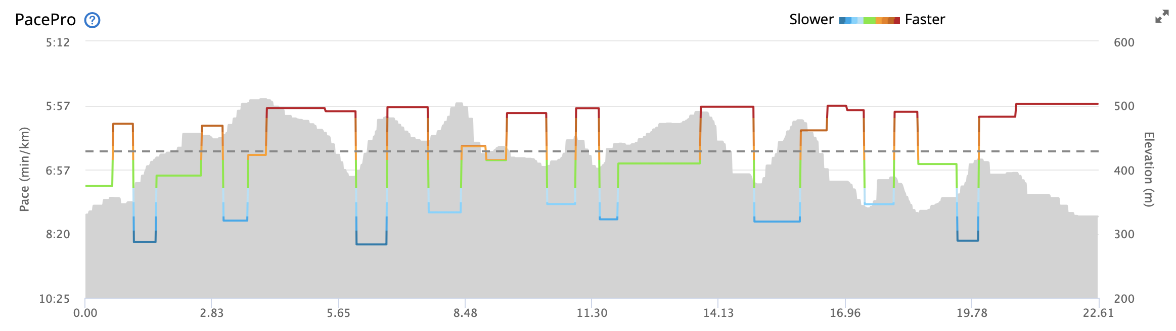
One challenge with trail running is that the pace of course depends on your fitness, but more so on conditions like elevation gain or surface of the trail. Hence, the available pacing strategies that rely on extrapolation of shorter distances do not work very well. Even more advanced approaches like Garmin’s PacePro(TM) do not consider all factors relevant for trail running as the impact of the surface of a trail cannot be configured in the UI and the impact of elevation can only be configured within bounds which are too limited for steep uphill or technically challenging downhill passages. This example shows Garmin’s pacing strategy for the quite challenging GebürgTrail in Franconia. For someone running at 6:00min/km pace on even grounds, 8:00 to 9:00 min/km pace on the steep ascents of the GebürgTrail is not feasible at all.

So why not base the pace prediction on your personal experiences on the trail. This is exactly what this little project is doing: based on a previous run (hereafter referred to as “reference run”) on similar terrain with comparable elevation and surface, a pacing strategy for a future run is provided (hereafter referred to as “target run”, e.g. an upcoming ultra marathon race).

This blog post gives a brief overview of the implementation of the “Pace Predictor” and allows you to further adjust or improve the implementation to your own needs. The main sections of this post are:

• Data Loading Reference Run

• Data Preparation

• Creation of the Model

• Data Loading Target Run

• Application of the Model

The full source code is avail on GitHub and advanced readery may prefer to just read this Jupyter Notebook instead of this chatty blog post.

Data Loading Reference Run

The reference run is provided as a GPX file with a GPS track and respective timings. This implementation uses the gpxpy library for procession the GPX file format. The data is collected in an array and then converted in a Pandas data frame.

import gpxpy
import gpxpy.gpx

gpx_file = open('data/osterfeld.gpx', 'r')
gpx = gpxpy.parse(gpx_file)

cols = [ 'lat', 'lon', 'elevation', 'time' ]
idx = []
rows = []

row = 0
for track in gpx.tracks:
    for segment in track.segments:
        for point in segment.points:
            idx.append(row)
            rows.append([point.latitude, point.longitude, point.elevation, point.time])
            row = row + 1
            
base = pd.DataFrame(data=rows, index=idx, columns=cols)

Data Preparation

The data provided in the GPX file is just a series of discrete points. So to turn this into a continuous stream of data, some additional fields need to be calculated:

• Elevation Delta: The difference in elevation to the previous track point.

• Time Delta: The time difference to the previous track point (Note: With a Garmin Fenix 6 in hires recording, this is always one second).

• Distance Delta: The distance to the previous track point (line of sight).

• Distance Sum: The accumulated distance of the track up to this trackpoint.

• Distance Segment: The number of the 100m segment this trackpoint belongs to.

base['elevation_delta'] = 
    base.elevation.diff().shift(0)
base['time_prev'] = 
    base.time.shift(+1)
base['time_delta'] = 
    base.apply(lambda row: time_delta(row['time'],row['time_prev']), axis=1)
base['lat_prev'] = 
    base.lat.shift(+1)
base['lon_prev'] = 
    base.lon.shift(+1)
base['distance_delta'] = 
    base.apply(lambda row: 
        distance(row['lat'],row['lon'],row['lat_prev'],row['lon_prev']), axis=1)
base['distance_sum'] = 
    base['distance_delta'].cumsum(axis = 0)
base['distance_segment'] = 
    base.apply(lambda row: distance_to_segment(row['distance_sum']), axis=1)

As a next step we group the track points by 100m segments and create a data frame that gives us elevation and timings for each segment. We also convert speed (in m/s) in pace (in min/km).

base_g = 
    base.groupby('distance_segment').agg(
        {
            'elevation_delta': ['sum'],
            'distance_delta': ['sum'], 
            'time_delta': ['sum']})
base_g['pace_segment'] = 
    16.7/(base_g[('distance_delta','sum')]/base_g[('time_delta','sum')])

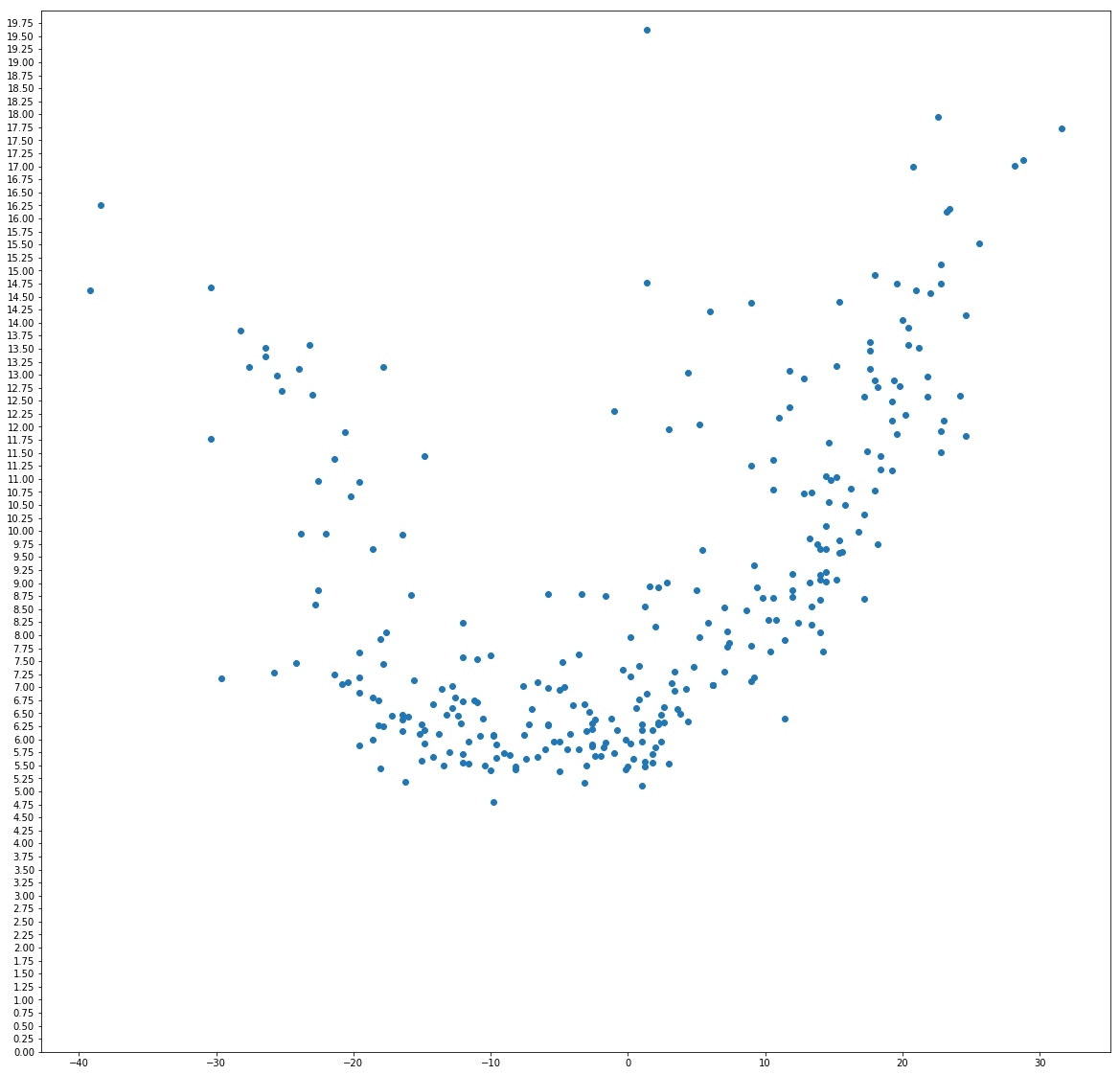
When plotting the result it becomes evident that the pace per segment depends on the elevation gain (or loss) of the segment with slight elevation losses still speeding up the base pace, but steeper decents also take their toll on the pace.

Creation of the Model

Based on the data prepared from the reference run, we can now train simple regression models (marketing speak: machine learning models!). Based on the visual inspection of the data, one could either use two linear regression models (there is a different slope for uphill and downhill) or a parabolic regression model, or a combination of both.

Hence we create data sets for uphill, downhill, and both.

base_g_sorted = base_g.sort_values(by=('elevation_delta','sum'))
x_arr = base_g_sorted[('elevation_delta','sum')].values
y_arr = base_g_sorted['pace_segment'].values

x_all_arr = []
y_all_arr = []
x_up_arr = []
y_up_arr = []
x_down_arr = []
y_down_arr = []

for i in range(0, len(x_arr)):
    if y_arr[i] < 20:
        x_all_arr.append(x_arr[i])
        y_all_arr.append(y_arr[i])
        if x_arr[i] > 0:
            x_up_arr.append(x_arr[i])
            y_up_arr.append(y_arr[i])
        else:
            x_down_arr.append(x_arr[i])
            y_down_arr.append(y_arr[i])

Now the creation of the models is pretty straight forward.

(a_para,b_para,c_para) = polyfit(x_all_arr, y_all_arr, 2)
(a_lin_up,b_lin_up) = polyfit(x_up_arr, y_up_arr, 1)    
(a_lin_down,b_lin_down) = polyfit(x_down_arr, y_down_arr, 1)
(a_para_down,b_para_down,c_para_down) = polyfit(x_down_arr, y_down_arr, 2)

When reviewing the models against the points representing the individual segments, we see a relatively good fit for all aproaches.

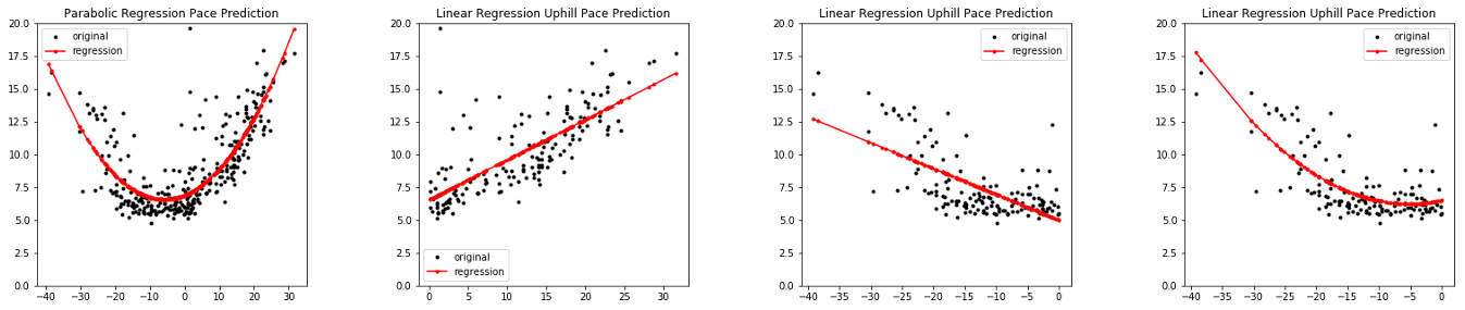
For now, we do not commit to one particular model, but create a wrapper function, that allows the selection of a model at runtime. For checking, a manual linear model has been hard-coded as well.

uphill_penalty_per_m=6/20
downhill_penalty_per_m=3/20

def predict_pace_raw(elevation, base_pace, model):
    if model=='manual':
        if elevation > 0:
            return base_pace+elevation*uphill_penalty_per_m
        else:
            return base_pace+abs(elevation)*downhill_penalty_per_m

    elif model=='parabolic':
        return a_para*elevation**2+b_para*elevation+c_para
    
    elif model=='linear':
        if elevation >= 0:
            return a_lin_up*elevation+b_lin_up
        else:
            return a_lin_down*elevation+b_lin_down
    
    elif model=='mixed':
        if elevation > 0:
            return a_lin_up*elevation+b_lin_up
        else:
            return a_para_down*elevation**2+b_para_down*elevation+c_para_down
        
def predict_pace(elevation, base_pace, model, min_pace=19):
    pace = predict_pace_raw(elevation, base_pace, model)
    if pace > min_pace:
        return min_pace
    else:
        return pace

Data Loading Target Run

Preparing the target run follows the same approaches used for the reference run.

target_gpx_file = open('data/supertrail.gpx', 'r')
target_gpx = gpxpy.parse(target_gpx_file)

cols = [ 'lat', 'lon', 'elevation' ]
idx = []
rows = []

row = 0
for track in target_gpx.tracks:
    for segment in track.segments:
        for point in segment.points:
            idx.append(row)
            rows.append([point.latitude, point.longitude, point.elevation])
            row = row + 1

target = pd.DataFrame(data=rows, index=idx, columns=cols)

Accodringly, additional columns are prepared and the data frame is grouped.

target['elevation_delta'] = 
    target.elevation.diff().shift(0)
target['lat_prev'] = 
    target.lat.shift(+1)
target['lon_prev'] = 
    target.lon.shift(+1)
target['distance_delta'] = 
    target.apply(
        lambda row: distance(row['lat'],row['lon'], row['lat_prev'],row['lon_prev']), axis=1)
target['distance_sum'] = 
    target['distance_delta'].cumsum(axis = 0)
target['distance_segment'] = target.apply(
    lambda row: distance_to_segment(row['distance_sum']), axis=1)

target_g = target.groupby('distance_segment').agg(
    {
        'elevation': ['mean'],
        'elevation_delta': ['sum'],
        'distance_delta': ['sum']})

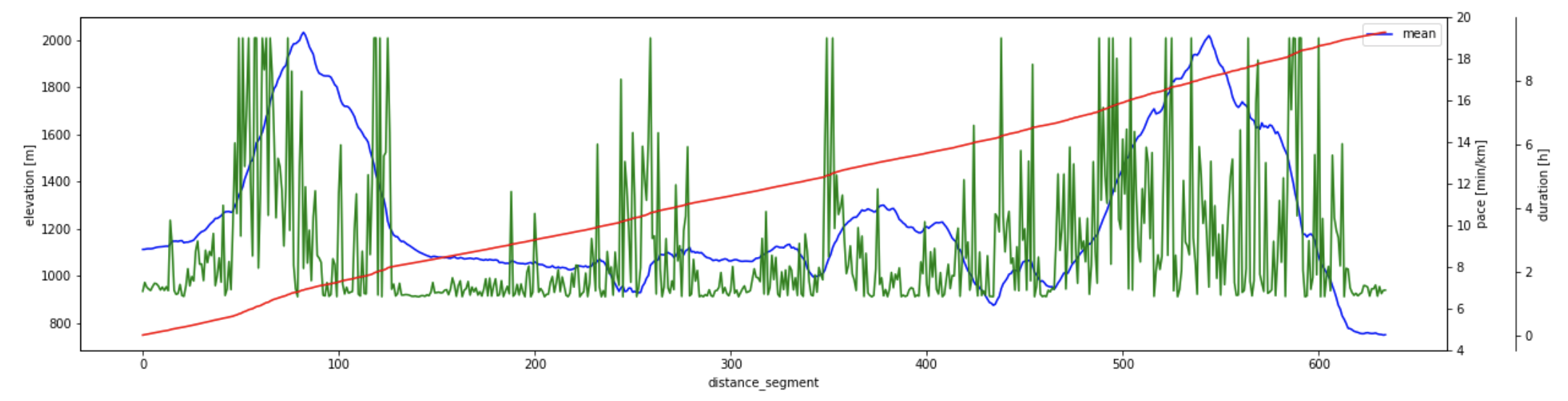
Application of the Model

Now everything gets very simple (as always when you are well prepared):

target_g['pace_segment'] = target_g.apply(
    lambda row: predict_pace(row[('elevation_delta','sum')], 6.5, 'parabolic'), axis=1)

target_g['time_delta'] = target_g[('distance_delta','sum')]/(16.7/target_g['pace_segment'])
target_g['time_sum'] = target_g['time_delta'].cumsum(axis = 0)/3600

And we create the final plot, where multiple dimensions are put together in a single diagram:

fig,ax = plt.subplots()

ax.set_ylabel('elevation [m]')
ax.set_xlabel('segments [100m]')

ax2 = ax.twinx()
ax2.set_ylim(4, 20)
ax2.set_ylabel('pace [min/km]')
ax3 = ax.twinx()
rspine = ax3.spines['right']
rspine.set_position(('axes', 1.05))
ax3.set_frame_on(True)
ax3.patch.set_visible(False)
ax3.set_ylabel('duration [h]')


target_g['elevation'].plot(ax=ax, style='b-', figsize=(20,5))
target_g['pace_segment'].plot(ax=ax2, style='g-')
target_g['time_sum'].plot(ax=ax3, style='r-')